Inventory Demand Forecasting: A Practical Guide for US Supply Chains
Inventory Demand Forecasting: A Practical Guide for US Supply Chains
The fastest route to lower stockouts and holding costs is an SKU-by-location probabilistic demand forecast tied directly to replenishment rules — Economic Order Quantity, reorder point, and safety stock — with machine learning demand sensing layered in where your data volume supports it. That combination outperforms either approach alone, and the research backs it: accurate forecasting paired with real-time data has reduced stockouts by a significant margin in documented industry deployments. The right place to start is a three-month pilot on your top 100 SKUs across one to three locations.
Start this week:
- Pull two or more years of daily sales history at SKU×location and flag any gaps or outliers
- Run a naive baseline forecast (moving average or EWMA) to establish your current MAPE and MAE
- Define pilot scope: 100 highest-velocity SKUs, one to three locations, 13-week horizon
Key Takeaways
Accurate inventory demand forecasting requires probabilistic SKU-by-location forecasts, formula-driven replenishment rules, and continuous reforecasting — with ML demand sensing added where data volume justifies it.
| Point | Details |
|---|---|
| Start with a scoped pilot | Run 100 top-velocity SKUs across 1–3 locations for 13 weeks before scaling. |
| Anchor on EOQ, ROP, safety stock | Calibrated replenishment formulas convert forecast outputs into real order decisions. |
| Match method to SKU pattern | Use ARIMA or Prophet for seasonal SKUs; XGBoost for promotion-heavy items; Croston for intermittent demand. |
| Measure MAPE, MAE, and bias by segment | Aggregate accuracy scores hide failures in slow-moving or high-value SKUs. |
| Arosplatforms for production deployment | Arosplatforms embeds within operations to take forecasting programs from pilot to ERP-integrated production, with many clients seeing ROI within twelve months. |
Table of Contents
- What is inventory demand forecasting, and how does it differ from demand forecasting?
- Why better forecasts translate directly to lower costs
- Which forecasting methods should you actually use?
- Key inventory formulas and how to apply them
- What data do you need, and how do you engineer features?
- How to implement a forecasting program, step by step
- What tools and architecture do you need?
- How to validate forecasts and avoid the most common mistakes
- How Arosplatforms applies AI to inventory demand forecasting
- The part most forecasting guides get wrong
- Arosplatforms builds forecasting systems that actually ship to production
- Key Takeaways
- Sources
- FAQ
What is inventory demand forecasting, and how does it differ from demand forecasting?
These two terms get used interchangeably in most planning meetings, but they describe different problems. Demand forecasting is an independent forecast: it predicts what customers will want, based on sales history, seasonality, promotions, and external signals. Inventory forecasting is a derivative forecast — it takes that demand signal and converts it into replenishment schedules, warehouse capacity plans, and purchase order timing.
The distinction matters because the two forecasts operate at different granularities and horizons. A demand forecast might run at the product-category level for a 12-month S&OP cycle. An inventory forecast runs at SKU×location, often daily, to answer a narrower question: when do I order, how much, and where does it need to be?
| Forecast type | Typical horizon | Granularity | Primary output |
|---|---|---|---|
| Demand forecast | 1–12 months | Category / SKU | Expected units sold |
| Inventory forecast | 1–7 days | SKU × location | Replenishment order qty |
| S&OP / IBP | 3–18 months | Product family | Capacity and budget plan |
| Daily replenishment | 1–7 days | SKU × DC / store | Purchase or transfer order |
A separate inventory model becomes necessary when lead-time variability is high, when you carry thousands of SKUs across multiple distribution centers, or when your demand forecast horizon is longer than your replenishment cycle. In those cases, a single aggregate forecast will systematically under-stock fast movers and over-stock slow ones.
Why better forecasts translate directly to lower costs
Stockouts and excess inventory are both expensive, and they usually coexist in the same warehouse. The root cause is almost always a forecast that is either too coarse, too stale, or both.
The business case for fixing this is concrete:
- Stockout reduction: Real-time, synchronized forecasting has cut stockout rates by 20–50% in documented deployments — a direct hit to lost sales and emergency expedite costs
- Carrying cost reduction: Tighter safety stock calibration, driven by accurate demand variability estimates, reduces excess inventory and the capital tied up in it
- Service level improvement: Higher forecast accuracy translates to a measurable fill-rate lift, which matters for customer retention and contract compliance
- Working capital: Lower average inventory frees cash for other uses without sacrificing availability
- Obsolescence and markdown reduction: Better visibility into slow-moving SKUs lets you act before product ages out
A sensor-enabled retail study combining transformer-based forecasting with multi-agent reinforcement learning reported roughly 18.2% lower forecast error and 23.5% fewer stockouts versus state-of-the-art baselines.
To translate forecast improvements into P&L language, map MAPE reduction to fill-rate improvement using your service-level curve, then multiply fill-rate gain by your average lost-sale margin. Carrying cost savings come from the reduction in average cycle stock and safety stock. Bring finance, supply planning, and commercial teams into that calculation early — it builds the internal case for the investment and sets the KPIs you will track.
Which forecasting methods should you actually use?
The right method depends on your data volume, SKU mix, and how much promotional or seasonal complexity you carry. No single model wins everywhere.
Statistical baselines and smoothing
Moving averages and exponentially weighted moving averages (EWMA) are fast to implement and surprisingly hard to beat on stable, high-velocity SKUs with little seasonality. They belong in every forecaster’s toolkit as a baseline benchmark. If your ML model cannot beat EWMA on a given SKU segment, it is not ready for production.
ARIMA and SARIMA handle trend and seasonality explicitly through autoregressive and moving-average components. They work well on SKUs with clear seasonal patterns and at least two years of clean history. The downside is that each SKU needs its own fitted model, which creates maintenance overhead at scale.
Decomposition and open-source libraries
Prophet, Facebook’s open-source forecasting library, decomposes time series into trend, seasonality, and holiday components. It handles missing data and outliers gracefully, and its additive model structure makes it easy to incorporate known events like promotions or store closures. For retail and CPG teams running hundreds to thousands of SKUs, Prophet is often the fastest path from raw data to a defensible baseline.
Machine learning and feature-driven models
XGBoost and LightGBM treat forecasting as a supervised regression problem: you engineer lag features, rolling statistics, calendar flags, and promotion indicators, then train a gradient-boosted tree to predict future demand. These models capture non-linear interactions between features that ARIMA cannot — for example, the combined effect of a price cut during a holiday week. They require more data engineering but tend to outperform statistical models on SKUs with rich feature sets and promotional complexity.
Hybrid approaches that combine statistical baselines with ML demand sensing are widely recommended for handling promotions, seasonality, and shifting market conditions simultaneously. A common pattern: use ARIMA or Prophet for the base trend-seasonal signal, then use XGBoost residuals to capture promotion lifts and external drivers.
Decision framework
| Scenario | Recommended approach |
|---|---|
| Stable, high-velocity SKUs, minimal promotions | EWMA or ARIMA |
| Strong seasonality, holiday effects, clean history | Prophet |
| Rich feature data, promotions, price changes | XGBoost / LightGBM |
| Sparse or intermittent demand | Croston’s method or bootstrapped aggregation |
| Large SKU catalog, mixed patterns | Ensemble: statistical base + ML residual correction |
| Near-real-time demand sensing | ML with rolling retraining on recent windows |
Key inventory formulas and how to apply them
These formulas convert a demand forecast into actual order decisions. Get them right and your forecast accuracy gains show up in inventory levels. Get them wrong and even a perfect forecast produces the wrong orders.
| Metric | Formula |
|---|---|
| Economic Order Quantity (EOQ) | √(2 × D × S / H) |
| Reorder Point (ROP) | (Average daily demand × Lead time) + Safety stock |
| Safety stock | Z × σ_demand × √Lead time |
| Lead-time demand | Average daily demand × Lead time |
| Inventory turnover | COGS / Average inventory value |
| MAPE | Mean of |
| MAE | Mean of |
Variables: D = annual demand (units), S = ordering cost per order ($), H = holding cost per unit per year ($), Z = service-level Z-score (e.g., 1.65 for 95%), σ_demand = standard deviation of daily demand.
Worked example: EOQ and ROP for a single SKU
- Inputs: Annual demand D = 12,000 units; ordering cost S = $150; holding cost H = $6/unit/year; average daily demand = 33 units; lead time = 7 days; σ_demand = 8 units/day; target service level = 95% (Z = 1.65)
- EOQ: √(2 × 12,000 × 150 / 6) = √600,000 = 775 units per order
- Safety stock: 1.65 × 8 × √7 = 1.65 × 8 × 2.65 = 35 units
- ROP: (33 × 7) + 35 = 231 + 35 = 266 units
- Interpretation: Place a new order of 775 units whenever on-hand inventory drops to 266 units.
On forecast accuracy metrics: MAPE is the default, but it breaks down for intermittent or near-zero demand SKUs because small actual values inflate the percentage error. For sparse SKUs, use MAE or weighted MAPE instead. Track bias (mean of Forecast − Actual) separately from error magnitude — a forecast that is consistently 10% high is a different problem than one that is randomly wrong by 10%.
What data do you need, and how do you engineer features?
Model quality is a direct function of data quality. A sophisticated XGBoost model fed dirty data will underperform a simple moving average fed clean data.
Required data:
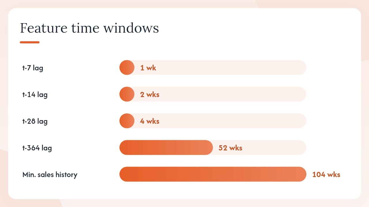
- Daily or weekly sales history at SKU×location, minimum 104 weeks (two years) for seasonal models
- Current on-hand inventory, in-transit stock, and outstanding POs
- Supplier lead times and lead-time variability (standard deviation, not just average)
- Promotion calendar: dates, depth of discount, and affected SKUs
- Price history at SKU level
Helpful enrichment data:
- Store or DC attributes (size, region, channel type)
- Public holidays and local events
- Weather data for weather-sensitive categories
- Economic indicators (consumer confidence, fuel prices for logistics-heavy SKUs)
- Web traffic or search trend data as a leading indicator
Feature engineering for ML models:
- Lag features: sales at t-7, t-14, t-28, t-364 (same week prior year)
- Rolling aggregates: 4-week and 13-week rolling mean and standard deviation
- Calendar flags: day of week, week of year, holiday binary, days-to-holiday
- Promotion encoding: is_promo binary, discount depth as a continuous feature
- Price elasticity signals: log(price) or price relative to 52-week average
Pro Tip: For intermittent or slow-moving SKUs — parts inventory, seasonal accessories, low-velocity B/C items — standard time-series models produce noisy, unreliable forecasts. Use Croston’s method, which separates the frequency of demand from the size of each demand event, or apply bootstrap aggregation across similar SKUs. The AI parts inventory guide from Arosplatforms covers this pattern in detail for automotive and industrial contexts.
For data gaps, use forward-fill for short outages (one to three days) and flag longer gaps as missing rather than zero — zero sales during a stockout is not zero demand, and training a model on it will systematically underforecast.
How to implement a forecasting program, step by step
A forecasting program fails more often from poor rollout than from poor models. The sequence below keeps early wins visible and limits the blast radius of early mistakes.
Phase 1: Foundation (weeks 1–4)
- Audit data completeness: sales history, lead times, promotions, and on-hand inventory at SKU×location
- Define pilot scope: 50–200 SKUs, one to three locations, 13-week forecast horizon
- Establish baseline metrics: compute current MAPE, MAE, and bias using a naive or moving-average model
- Assign owners: data engineering (data pipelines), demand planners (model review and override), supply planners (replenishment rules), IT (integration and MLOps)
Phase 2: Pilot (weeks 5–12)
- Build and train candidate models (ARIMA, Prophet, XGBoost) on the pilot SKU set
- Run rolling-origin backtests over the last 13–26 weeks; compare MAPE/MAE against baseline
- Set EOQ, ROP, and safety stock parameters using pilot forecast outputs
- Present results to demand planners; collect override feedback and document reasons
Phase 3: Deploy and integrate (weeks 13–20)
- Deploy winning model to production with automated retraining cadence (weekly or biweekly)
- Connect forecast outputs to ERP or WMS replenishment module via API or flat-file export
- Integrate with S&OP cycle: feed 4–13 week forecasts into weekly planning meetings
- Set up monitoring dashboard: MAPE, MAE, bias, service level, and forecast value-add vs. baseline
Phase 4: Scale and improve (ongoing)
- Expand SKU and location coverage in quarterly waves
- Add enrichment features (promotions, weather, economic indicators) as data becomes available
- Review model performance monthly; retrain or recalibrate when bias exceeds a defined threshold
A pilot typically runs 8–12 weeks. Full rollout across a mid-sized SKU catalog (5,000–20,000 SKUs) usually takes 6–12 months depending on data readiness and ERP complexity. Continuous reforecasting — not a once-a-month batch run — is what keeps the system accurate as demand patterns shift.
Monitoring checklist:
- MAPE and MAE by SKU segment (A/B/C velocity tiers) weekly
- Bias trend: flag any segment where bias exceeds ±5% for three consecutive weeks
- Service level (fill rate) monthly, compared against pre-pilot baseline
- Forecast value-add: does the model beat the naive baseline? If not, investigate
What tools and architecture do you need?
The architecture does not need to be complex to be effective. The core pipeline looks like this:
Data sources → Feature store → Forecasting engine → Decision rules → ERP/WMS → Dashboards
Data sources feed cleaned, versioned features into a central store. The forecasting engine trains and scores models against those features. Decision rules (EOQ, ROP, safety stock) convert probabilistic forecasts into order recommendations. Those recommendations push into your ERP or WMS for execution, and a dashboard closes the loop with performance monitoring.
Tool categories:
- Forecasting libraries: Prophet (seasonal decomposition, holiday handling), statsmodels (ARIMA/SARIMA), sktime (unified time-series API)
- ML frameworks: XGBoost, LightGBM (gradient boosting), TensorFlow or PyTorch (sequence models for large catalogs)
- Orchestration and MLOps: Apache Airflow (pipeline scheduling), MLflow (experiment tracking and model registry), Kubeflow (Kubernetes-native ML pipelines)
- Feature stores: Feast (open-source), Tecton (managed), or a simple versioned table in your data warehouse
- ERP/WMS connectors: SAP IBP, Oracle SCM Cloud, NetSuite, or custom API/EDI integrations
| Layer | Open-source option | Managed/enterprise option |
|---|---|---|
| Forecasting | Prophet, statsmodels | AWS Forecast, Azure ML |
| ML training | XGBoost, LightGBM | Databricks, SageMaker |
| Orchestration | Airflow, Prefect | Astronomer, Kubeflow |
| Feature store | Feast | Tecton, Vertex AI Feature Store |
| ERP integration | Custom API / EDI | SAP IBP, Oracle SCM |
One architecture pattern worth noting: LLM-as-Parser systems paired with constrained optimizers can translate natural-language demand signals or planner overrides into structured replenishment constraints — a practical way to keep human judgment in the loop without breaking the automated pipeline.
Integration tips: Sync lead-time and PO data from your ERP into the feature store on the same cadence as your retraining cycle. Maintain feature parity between training and production — a mismatch here is the most common cause of model degradation after deployment. Build a planner override layer so demand planners can adjust forecasts before they trigger orders, and log every override with a reason code for future model improvement.
How to validate forecasts and avoid the most common mistakes
A model that looks good in development and fails in production is the norm, not the exception. Validation discipline is what separates forecasting programs that stick from ones that get abandoned after six months.
Validation checklist:
- Rolling-origin (walk-forward) backtest over at least 13 weeks of held-out data
- Forecast value-add test: does the model beat a naive baseline (last year same week) on MAPE?
- Segment-level diagnostics: break MAPE and bias down by SKU velocity tier (A/B/C) and by location
- Residual analysis: check for autocorrelation in errors, which signals a missing feature or wrong model family
- Service-level simulation: translate forecast error distribution into expected fill rate at your target safety stock
Common pitfalls and how to fix them
- Wrong granularity: Forecasting at the category level and disaggregating to SKU×location introduces systematic error. Build at the level you replenish.
- Ignoring lead-time variability: Using average lead time in your ROP formula without accounting for variability understates safety stock. Use the standard deviation of lead time in your safety stock calculation.
- Overfitting to promotions: Including promotion features without a proper holdout that contains promotions produces models that look accurate in training and fail on future events. Always include at least two promotional periods in your test set.
- Poor data hygiene: Zero sales during a stockout period, duplicate transactions, and unit-of-measure mismatches will corrupt any model. Audit before you train.
- Misreading MAPE on sparse SKUs: MAPE is undefined at zero actuals and misleading near zero. Switch to MAE or weighted absolute percentage error for intermittent items. The AI parts inventory guide covers intermittent-SKU handling in depth.
Mitigations:
- Segment your SKU catalog by demand pattern (smooth, erratic, intermittent, lumpy) and assign model families per segment
- Use a robust holdout design: the test period must include the same seasonal and promotional conditions you expect in production
- Set a bias alert threshold (±5% for three consecutive weeks) and trigger a model review automatically
- Schedule quarterly model recalibration as a standing agenda item in your S&OP process
How Arosplatforms applies AI to inventory demand forecasting
The gap between a working prototype and a production forecasting system that planners actually trust is where most internal projects stall. Arosplatforms closes that gap by embedding directly within client operations rather than handing over a model and walking away.
A typical engagement runs through four phases:
- Discovery (weeks 1–3): Data audit, stakeholder interviews, current-state MAPE baseline, and pilot scope definition
- Pilot (weeks 4–12): Model development (ARIMA, Prophet, XGBoost candidates), backtesting, EOQ/ROP calibration, and planner review sessions
- Deploy (weeks 13–20): Production deployment, ERP/WMS integration, MLOps setup (Airflow, MLflow), and S&OP integration
- Optimize (ongoing): Monthly model reviews, bias monitoring, feature expansion, and governance documentation
The team typically includes data engineers (pipeline and feature store), ML engineers (model training and MLOps), and supply-chain consultants (replenishment rules, S&OP alignment, and change management). That last role is the one most internal teams understaff.
Arosplatforms reports that many clients achieve ROI within twelve months, with substantially faster turnaround on key planning tasks after deployment.
The AI supply chain forecasting practice at Arosplatforms covers both demand sensing and inventory optimization, with documented experience across logistics, manufacturing, and retail. For teams that need to move from pilot to production without building an internal ML team from scratch, that combination of embedded consulting and owned infrastructure is the practical path.
The part most forecasting guides get wrong
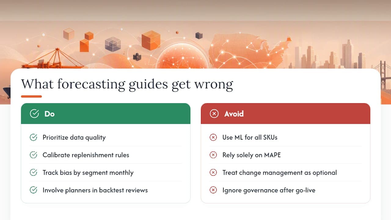
Most guides on demand forecasting spend the bulk of their pages on model selection — ARIMA vs. Prophet vs. XGBoost — as if picking the right algorithm is the hard part. It is not. The hard part is the 80% of work that happens before and after the model: data quality, replenishment rule calibration, planner adoption, and the governance that keeps the system accurate six months after go-live.
The conventional advice also overstates the case for ML. For the majority of SKUs in a typical US distribution operation — stable, high-velocity items with two or more years of clean history — a well-tuned ARIMA or Prophet model will match or beat XGBoost, at a fraction of the maintenance cost. ML earns its keep on the SKUs with rich feature sets: heavy promotional activity, price sensitivity, or external demand drivers. Applying it uniformly across a catalog is how teams end up with expensive infrastructure and marginal accuracy gains.
The other underrated lever is bias. Most teams track MAPE and call it done. But a forecast that is consistently 15% high on a specific product family is quietly inflating your safety stock and tying up working capital every single week. Bias by segment, reviewed monthly, is the metric that actually drives inventory cost reduction. Build that into your S&OP cadence before you invest in a more complex model.
Finally: change management is not a soft skill add-on. A forecasting system that planners do not trust will be overridden into irrelevance within three months. The pilot phase exists partly to build that trust — not just to validate the model. Involve planners in the backtest review, let them see where the model beats their intuition and where it does not, and give them a documented override process. That investment pays back faster than any model upgrade.
Arosplatforms builds forecasting systems that actually ship to production
Most supply chain teams can build a working forecast model. Getting it into production, connected to your ERP, trusted by planners, and still accurate six months later is the part that requires a different kind of help.
Arosplatforms works with US enterprises to design and deploy custom AI forecasting systems that are owned by your team, not locked to a vendor. The engagement covers the full stack: data pipelines, model development, ERP and WMS integration, MLOps, and the S&OP change management that makes planners actually use the output. Many clients reach ROI within twelve months, with planning task turnaround accelerating by an average of 82% after deployment.
If your forecasting pilot is stalling at the production handoff, or your current system is accurate in testing but not in practice, talk to the Arosplatforms team about a scoped engagement.
Key Takeaways
Accurate inventory demand forecasting requires probabilistic SKU-by-location forecasts, formula-driven replenishment rules, and continuous reforecasting — with ML demand sensing added where data volume justifies it.
Sources
The references below support the claims and frameworks in this article. Read them in the order that matches your next step.
- Inventory Forecasting vs. Demand Forecasting: What’s the Difference?
- The complete guide to inventory forecasting: Benefits + best practices in 2024 - Cin7
- Multi-Agent Deep Reinforcement Learning for Integrated Demand Forecasting and Inventory Optimization in Sensor-Enabled Retail Supply Chains
FAQ
What is the difference between demand forecasting and inventory forecasting?
Demand forecasting predicts how much customers will buy; inventory forecasting is a derivative calculation that converts that demand signal into replenishment quantities, reorder points, and warehouse capacity plans. The two forecasts operate at different granularities and serve different decisions.
What are the four main types of demand forecasting?
The four common types are qualitative (expert judgment, market research), time-series (ARIMA, moving averages, exponential smoothing), causal (regression models using external drivers like price or promotions), and AI/ML-based (XGBoost, neural networks, hybrid ensembles). Most production systems combine two or more of these.
What is the 80/20 rule in inventory management?
In inventory management, the 80/20 rule — also called the Pareto principle — holds that roughly 80% of your revenue or stockout risk typically comes from 20% of your SKUs. Prioritizing forecast accuracy and safety stock calibration for that top 20% delivers most of the business impact.
When should you use MAPE vs. MAE to measure forecast accuracy?
Use MAPE for high-velocity SKUs where actual demand is consistently above zero; it gives an intuitive percentage error that is easy to communicate. Switch to MAE for intermittent or slow-moving SKUs, where near-zero actuals inflate MAPE to the point of meaninglessness.
How does Arosplatforms help with inventory demand forecasting?
Arosplatforms designs and deploys custom AI forecasting systems that integrate with your ERP and WMS, covering data pipelines, model development, MLOps, and S&OP alignment. Many clients see ROI within twelve months, with key planning tasks completing 82% faster after deployment.
Recommended
Related: dispatch optimization systems.