AI Equipment Failure Prediction: A Practitioner's Guide
AI Equipment Failure Prediction: A Practitioner’s Guide
AI-driven equipment failure prediction, formally called predictive maintenance (PdM), uses sensor data and machine learning to estimate when a machine will fail before it actually does. The practical verdict: if you have sparse or no failure labels, start with anomaly detection; if you have run-to-failure histories, build a remaining useful life (RUL) model. Those two choices cover the vast majority of industrial programs.
Three things to do right now:
- Inventory your sensors — vibration, temperature, current, and pressure streams are the minimum viable signal set.
- Pick one target task — anomaly detection, fault classification, or RUL estimation; mixing all three in a first pilot is how programs stall.
- Run a small pilot on a single Tier-1 asset before committing to fleet-wide rollout.
RUL predictions are statistical estimates expressed as probability distributions with associated uncertainty, not single-point guesses. That distinction changes how maintenance planners schedule work and how engineers validate model outputs. Anomaly detection, fault classification, and RUL estimation are related but distinct problems, and conflating them is the most common reason industrial AI programs underdeliver.
Key Takeaways
AI equipment failure prediction succeeds when task selection, data quality, uncertainty quantification, and human-in-the-loop validation are treated as equally important as model choice.
| Point | Details |
|---|---|
| Match task to data availability | Use anomaly detection when failure labels are sparse; use RUL models only when run-to-failure histories exist. |
| Engineer features before modeling | RMS, kurtosis, FFT bins, and cross-sensor correlation features consistently outperform raw-stream inputs on small industrial datasets. |
| Quantify RUL uncertainty | Express RUL as a probability distribution with prediction intervals; a point estimate alone is insufficient for maintenance planning. |
| Deploy hybrid edge-cloud architecture | Run lightweight inference at the edge for low latency; retrain in the cloud on aggregated data with drift monitoring. |
| Adopt XAI from day one | SHAP attributions and signal-level evidence are prerequisites for operations team trust, not optional enhancements. |
Table of Contents
- What is AI-driven predictive maintenance, and how does it differ from preventive maintenance?
- How AI predicts failure: core tasks and the model families behind them
- What sensor data and features does AI failure prediction actually need?
- How do you match a failure mode to the right algorithm?
- How do you train, evaluate, and quantify uncertainty in PdM models?
- What deployment architecture and MLOps practices does a PdM system need?
- Why does explainability matter for PdM, and which XAI methods work in practice?
- A step-by-step checklist for running a PdM pilot
- Real-world examples: what AI failure prediction looks like in practice
- How Arosplatforms approaches PdM pilots in manufacturing
- The gap between model accuracy and operational adoption
- Sources
- FAQ
What is AI-driven predictive maintenance, and how does it differ from preventive maintenance?
AI-driven predictive maintenance uses real-time and historical sensor data, combined with machine learning models, to predict when a specific piece of equipment is likely to fail. The goal is to schedule maintenance at the last responsible moment, not on a fixed calendar.
Three tasks sit inside that umbrella:
- Anomaly detection: Identifies when a machine’s behavior deviates from its normal baseline. No failure label required. The model flags “something changed” without specifying what.
- Fault classification: Given labeled examples of specific failure modes (bearing spall, seal leak, winding fault), a supervised classifier identifies which fault is present and how severe it is.
- RUL estimation: Estimates how many operating hours, cycles, or days remain before a component crosses a failure threshold. Requires either run-to-failure data or a known degradation threshold.
Contrast that with the two older approaches. Reactive maintenance waits for failure, which maximizes asset utilization right up until an unplanned outage wipes out weeks of savings in a single emergency repair. Preventive maintenance runs on fixed schedules, which is safer but routinely replaces components that still have a significant portion of their useful life remaining. PdM sits between those extremes: it acts on evidence, not calendars or catastrophes.
The IIoT and AIoT infrastructure that makes PdM practical, connecting sensors to edge compute and cloud analytics, is now widely available. Platforms like Oracle’s cloud-based industrial AI offerings and tools like the MathWorks Predictive Maintenance Toolbox have lowered the barrier to entry considerably. The harder problem is usually data readiness, not compute access.
How AI predicts failure: core tasks and the model families behind them
The 2026 systematic review in Frontiers in Artificial Intelligence confirms what practitioners already suspect: algorithm selection depends almost entirely on task type. There is no universal “best” model for PdM. Here is how the major families map to the three core tasks.
Anomaly detection
Unsupervised and semi-supervised methods dominate here because labeled failure data is rarely available at program launch. Common choices include autoencoders (reconstruct normal behavior; high reconstruction error signals anomaly), Isolation Forest (partitions data; anomalies isolate quickly), and one-class SVMs. These models train on normal operating data only, which is almost always abundant.
Fault classification and diagnosis
Once failure labels exist, supervised classifiers take over. Random Forest and XGBoost handle tabular feature sets well and are fast to train and interpret. Convolutional neural networks (CNNs) excel at raw vibration spectrograms, learning frequency-domain patterns without manual FFT binning. LSTMs and temporal convolutional networks capture degradation sequences over time. Libraries: scikit-learn for classical ML, PyTorch and TensorFlow for deep learning.
RUL estimation and prognostics
Engineers can estimate RUL using three methodological families: degradation models, similarity models, and survival/proportional-hazard models, which are selected based on what data is available.
- Degradation models fit a parametric curve (exponential, polynomial) to a condition indicator and extrapolate to a threshold. Works when you know the failure threshold but have limited run-to-failure histories.
- Similarity models compare the current degradation trajectory to an ensemble of run-to-failure examples and estimate RUL by analogy. Requires a library of complete run-to-failure histories.
- Survival/proportional-hazard models use lifetime data and covariates to estimate failure probability over time. Useful when you have fleet-level lifetime data but not complete degradation curves.
The MathWorks Predictive Maintenance Toolbox implements all three families with named model objects (exponentialDegradationModel, pairwiseSimilarityModel, survival models) and supports recursive updates as new sensor data arrives.
Hybrid and physics-informed models
Pairing an unsupervised anomaly detector with a supervised RUL model is often the most practical architecture when labeled failure data is sparse. The detector flags candidates; the prognostic model estimates RUL only where labels exist. Physics-informed neural networks embed known degradation equations (Paris’ law for crack growth, Arrhenius for thermal aging) as constraints, which dramatically reduces the data needed to train a reliable model.
Pro Tip: Before reaching for a deep learning model, try an autoencoder trained on normal data alongside a simple Random Forest classifier on engineered features. In most industrial datasets, that hybrid outperforms a pure LSTM on the first iteration and is far easier to debug.
| Model family | Accuracy potential | Data requirement | Interpretability | Compute cost |
|---|---|---|---|---|
| Statistical/degradation models | Moderate | Low (threshold + trend) | High | Very low |
| Similarity models | Moderate–High | High (run-to-failure library) | Moderate | Low–Moderate |
| Classical ML (RF, XGBoost) | Moderate–High | Medium (labeled events) | Moderate–High | Low |
| Deep learning (CNN, LSTM) | High | High (large labeled sets) | Low | High |
| Hybrid/physics-informed | High | Low–Medium | Moderate | Moderate |
What sensor data and features does AI failure prediction actually need?
Data quality determines model quality more reliably than algorithm choice. Here is what matters in practice.
Common sensor types and their failure signals:
- Vibration (accelerometers): The primary signal for rotating machinery. Bearing defect frequencies, imbalance, and misalignment all appear in the frequency spectrum.
- Temperature (thermocouples, IR): Thermal runaway precedes many electrical and mechanical failures. Slow drift is as informative as sudden spikes.
- Motor current (current transformers): Current signature analysis detects rotor bar faults, eccentricity, and load changes without physical access to the machine.
- Pressure (transducers): Seal degradation, pump cavitation, and blockages show up as pressure fluctuations before catastrophic failure.
- Acoustic emission: High-frequency stress waves from crack propagation and surface fatigue, useful for slow-speed bearings where vibration signal-to-noise is poor.
- Oil analysis (particle counters, viscosity sensors): Wear debris concentration tracks gear and bearing wear over weeks to months.
Sampling rate matters. Vibration analysis for bearing defect frequencies typically requires 10–25 kHz continuous sampling. Temperature and pressure monitoring can run at 1 Hz or slower. Mixing high-rate and low-rate streams in the same pipeline requires careful resampling and alignment.
Run-to-failure vs. labeled failure events: Run-to-failure datasets record the full degradation trajectory from new to failed, which is what similarity and survival models need. Labeled failure events (a timestamp marking when a fault was confirmed) are sufficient for supervised classifiers but give no degradation trajectory. If you only have labeled events, start with classification; if you have complete run-to-failure histories, similarity and degradation models become viable.
Feature engineering that actually moves the needle:
- RMS (root mean square): Overall vibration energy; rises as bearing wear progresses.
- Kurtosis: Impulsiveness of the signal; spikes sharply when bearing spalls produce discrete impacts.
- Crest factor: Peak-to-RMS ratio; sensitive to early-stage defects before RMS rises.
- FFT bins at defect frequencies: Bearing outer-race, inner-race, and ball-pass frequencies computed from geometry and shaft speed.
- Cross-sensor correlation features: The correlation between vibration and temperature often changes before either sensor alone crosses a threshold.
A production-ready PdM pipeline built on these features, feeding an Isolation Forest and an autoencoder, demonstrates how feature engineering choices propagate through to serving and drift detection in a real deployment.
Pro Tip: Monitor cross-sensor correlation drift as a leading indicator. When vibration and temperature correlation breaks down, it often signals a developing fault days before either sensor’s individual threshold triggers. Most teams only watch single-sensor thresholds and miss this early warning.
How do you match a failure mode to the right algorithm?
The decision comes down to two variables: how many failure labels you have, and how far in advance you need to predict.
Decision matrix:
| Label availability | Failure horizon | Recommended approach |
|---|---|---|
| None (normal data only) | Imminent anomaly | Autoencoder, Isolation Forest, one-class SVM |
| Sparse labeled events | Short-term fault ID | Random Forest, XGBoost on engineered features |
| Run-to-failure histories | Long-term RUL | Similarity models, degradation models, survival analysis |
| Rich labeled + run-to-failure | Both horizons | Hybrid: anomaly detector + supervised RUL model |
Mapping common failure modes:
- Bearing faults: Vibration (FFT at defect frequencies, kurtosis), temperature. Early-stage: autoencoder anomaly detection. Confirmed fault: CNN classifier on spectrograms. Remaining life: similarity model against run-to-failure library.
- Seal leaks: Pressure drop trends, acoustic emission. Degradation model extrapolating pressure decay rate to a minimum acceptable threshold.
- Motor winding faults: Current signature analysis (FFT of current waveform at sideband frequencies), temperature. Supervised classifier (XGBoost or Random Forest) once labeled examples exist.
When labeled data is sparse but run-to-failure data exists for a similar machine type, transfer learning is worth attempting. The Frontiers 2026 systematic review identifies knowledge-transfer approaches as critical for robustness in real deployments, particularly when fleet diversity makes single-model generalization unreliable.
How do you train, evaluate, and quantify uncertainty in PdM models?
Evaluation for PdM is not the same as standard ML benchmarking. Time-series structure, class imbalance, and the cost asymmetry between false alarms and missed failures all require deliberate choices.
Metrics by task:
- Fault classification: Precision, recall, F1-score (weight recall heavily when missed failures are costly), ROC-AUC for threshold-independent comparison.
- Anomaly detection: Precision@k (are the top-k flagged instances actually anomalous?), false alarm rate (FAR), and detection lead time.
- RUL estimation: MAE and RMSE on held-out run-to-failure trajectories, plus timeliness metrics that penalize late predictions more than early ones.
- Business KPIs: Mean time to repair (MTTR) reduction, unplanned downtime hours avoided, and maintenance cost per operating hour.
Uncertainty quantification for RUL: A point estimate of “142 hours remaining” is nearly useless for maintenance planning. A probability distribution over RUL, showing the 10th, 50th, and 90th percentile, lets planners decide whether to act conservatively (schedule at the 10th percentile) or accept more risk. Conformal prediction methods wrap any trained model and produce statistically valid prediction intervals without retraining.
Key insight on RUL outputs: When a model’s RUL distribution is wide (high uncertainty), that is information, not a failure. It means the model needs more data from this specific degradation trajectory, and the maintenance planner should schedule a closer inspection rather than waiting for the median estimate.
Validation for time-series data: Never shuffle time-series data for cross-validation. Use walk-forward validation: train on all data up to time T, test on the window immediately after T, then advance T. For run-to-failure datasets, hold out complete machine lifetimes, not random time windows, to avoid data leakage from the same machine’s degradation trajectory appearing in both train and test sets.
Production-readiness checklist before go-live:
- False alarm budget defined and agreed with operations (e.g., no more than two false alarms per asset per month).
- Cost-sensitive decision thresholds set based on repair cost vs. failure cost ratio.
- Human-in-the-loop gate: model flags, human approves work order.
- Calibration check passed on held-out data.
What deployment architecture and MLOps practices does a PdM system need?
Architecture choice depends on latency requirements, connectivity, and data privacy constraints. Three patterns cover most industrial cases.
- Edge-only inference: Model runs on a gateway or PLC-adjacent device at the machine. Latency is milliseconds; no cloud dependency. Best for safety-critical applications or air-gapped OT networks. Constraint: limited compute for complex models; retraining requires manual update cycles.
- Cloud-only: All inference and retraining happen in the cloud. Easiest to maintain and scale; supports large models. Requires reliable connectivity and introduces latency (seconds to minutes). Acceptable for non-real-time RUL updates.
- Hybrid (edge inference + cloud retraining): The pragmatic production pattern. Lightweight models run at the edge for low-latency anomaly detection; full model retraining and RUL estimation happen in the cloud on aggregated data. AIoT architectures with edge inference, cloud retraining, and feedback loops are the standard for production PdM at scale. Arosplatforms’ AI infrastructure and MLOps practice for manufacturing is built around this hybrid pattern.
Streaming and ingestion: Industrial message buses (OPC-UA, MQTT) feed data to a streaming layer (Apache Kafka or a managed equivalent). For intermittent connectivity, local buffering with store-and-forward prevents data loss during network outages.
MLOps concerns:
- Drift detection: Monitor feature distributions and model output distributions over time. A shift in the vibration RMS baseline after a maintenance event is expected; a gradual shift without a maintenance event is a warning sign.
- Retraining cadence: Trigger-based retraining (drift threshold crossed) outperforms fixed-schedule retraining in most industrial settings.
- Experiment tracking: Use MLflow or a comparable tool to version models, datasets, and hyperparameters. Rollback to a previous model version must be a one-step operation.
- CMMS integration: Model alerts should automatically generate draft work orders in the CMMS (SAP PM, IBM Maximo, or equivalent). Alert throttling prevents alarm flooding; a single asset should not generate more work orders than the maintenance team can realistically process.
Tradeoffs to document before deployment:
- Edge compute adds hardware cost and a firmware maintenance burden.
- Cloud inference adds latency and ongoing compute cost.
- OT/IT network integration introduces cybersecurity exposure that requires review. Arosplatforms’ AI security practice for manufacturing addresses OT-specific threat modeling as part of deployment planning.
Why does explainability matter for PdM, and which XAI methods work in practice?
A 2026 IOP survey on explainable AI for RUL is direct: black-box models create trust and debugging barriers that prevent industrial adoption. A maintenance technician who cannot understand why a model flagged a bearing will override the alert. After enough overrides, the program dies regardless of model accuracy.
Practical XAI methods for industrial PdM:
- SHAP (SHapley Additive exPlanations): For tabular feature models (Random Forest, XGBoost), SHAP values show which features drove a specific prediction. Showing a technician that “kurtosis at 12.4 contributed 68% of the anomaly score” is actionable.
- Attention maps and feature importance for time-series: For LSTM and transformer models, attention weights highlight which time steps the model weighted most heavily. Visualizing these alongside the raw signal helps engineers validate that the model is responding to physically meaningful events.
- Surrogate models: A simple decision tree trained to approximate a complex model’s outputs provides a human-readable rule set for audit and debugging.
- Signal-level evidence: Always present the raw signal evidence alongside any model output. A spectrogram showing a growing peak at the bearing outer-race defect frequency is more persuasive to a maintenance engineer than any model confidence score.
Human-in-the-loop workflow: The model flags an anomaly or generates an RUL estimate. The operator reviews the signal evidence and the SHAP attribution. If the operator disagrees, that disagreement is logged and fed back into the retraining pipeline. This feedback loop is how models improve after deployment, and it is also how operations teams build trust in the system over time.
Pro Tip: Present RUL outputs as a confidence band, not a single number. Showing “failure in 110 hours” prompts an argument about whether the model is right.
A step-by-step checklist for running a PdM pilot
A pilot that tries to cover every asset and every failure mode simultaneously almost always fails. The following sequence keeps scope tight and delivers a go/no-go decision within a defined window.
- Scoping (weeks 1–2): Select one Tier-1 asset with known failure history. Define the target task (anomaly detection or RUL). Confirm sensor availability and data access. Document the business case (cost of one unplanned failure vs. pilot cost).
- Data ingestion and validation (weeks 3–5): Connect data streams, validate sampling rates, check for gaps and sensor drift. Run cross-sensor correlation analysis. Assess label availability. An AI readiness assessment at this stage prevents wasted modeling effort on inadequate data.
- Offline modeling and validation (weeks 6–10): Train candidate models on historical data. Evaluate with walk-forward validation. Quantify uncertainty for RUL outputs. Set false alarm budget and decision thresholds.
- Shadow deployment (weeks 11–14): Run the model in parallel with existing maintenance practice. Log all alerts without acting on them. Compare model alerts to actual maintenance events.
- Operator validation and go/no-go (week 15): Review shadow results with the maintenance team. If false alarm rate exceeds budget or RUL calibration is unstable, stop and diagnose before scaling. If results meet criteria, approve scale-up.
- Scale-up (months 4–6+): Extend to additional assets of the same type. Implement CMMS integration and drift monitoring. Plan retraining cadence.
Typical cost drivers: Sensor retrofits (the largest variable cost for older assets), edge compute hardware, CMMS integration development, and data labeling effort. PdM programs that leverage AI-driven parts inventory forecasting alongside failure prediction often see faster ROI because spare-parts costs drop in parallel with unplanned downtime.
Red flags that should stop scale-up:
- False alarm rate exceeds the agreed budget after threshold tuning.
- RUL prediction intervals are so wide they provide no scheduling value.
- Data gaps exceed 15% of the target operating period.
- Operations team consistently overrides model alerts without logging reasons.
Real-world examples: what AI failure prediction looks like in practice
Bearing vibration anomaly detection
A rotating machine with accelerometers sampled at 20 kHz generates vibration data continuously. Feature engineering extracts kurtosis, RMS, crest factor, and FFT bins at the bearing outer-race defect frequency (BPFO) and inner-race defect frequency (BPFI) for each shaft revolution. An autoencoder trained on 90 days of normal operation learns the baseline reconstruction. An Isolation Forest runs in parallel on the same feature set.
When a bearing begins to spall, kurtosis rises sharply while RMS lags. The autoencoder reconstruction error crosses its threshold first, typically 2–4 weeks before a conventional vibration alarm would trigger. The maintenance team receives a CMMS work order flagged as “bearing anomaly, inspect within 10 days.” The bearing is replaced during a planned outage rather than an emergency shutdown. Industry case studies document this pattern converting emergency repairs into planned outages with substantial cost savings.
RUL estimation for a wear-prone component
A hydraulic pump with a known seal degradation pattern accumulates run-to-failure data across a fleet of 40 identical units. A similarity model compares the current unit’s pressure-decay trajectory to the run-to-failure library and estimates RUL as a distribution. The 10th percentile of that distribution drives the maintenance schedule; the 90th percentile defines the latest acceptable intervention. As the pump ages, the model updates its estimate with each new pressure reading, narrowing the uncertainty band.
Edge IIoT deployment on constrained hardware
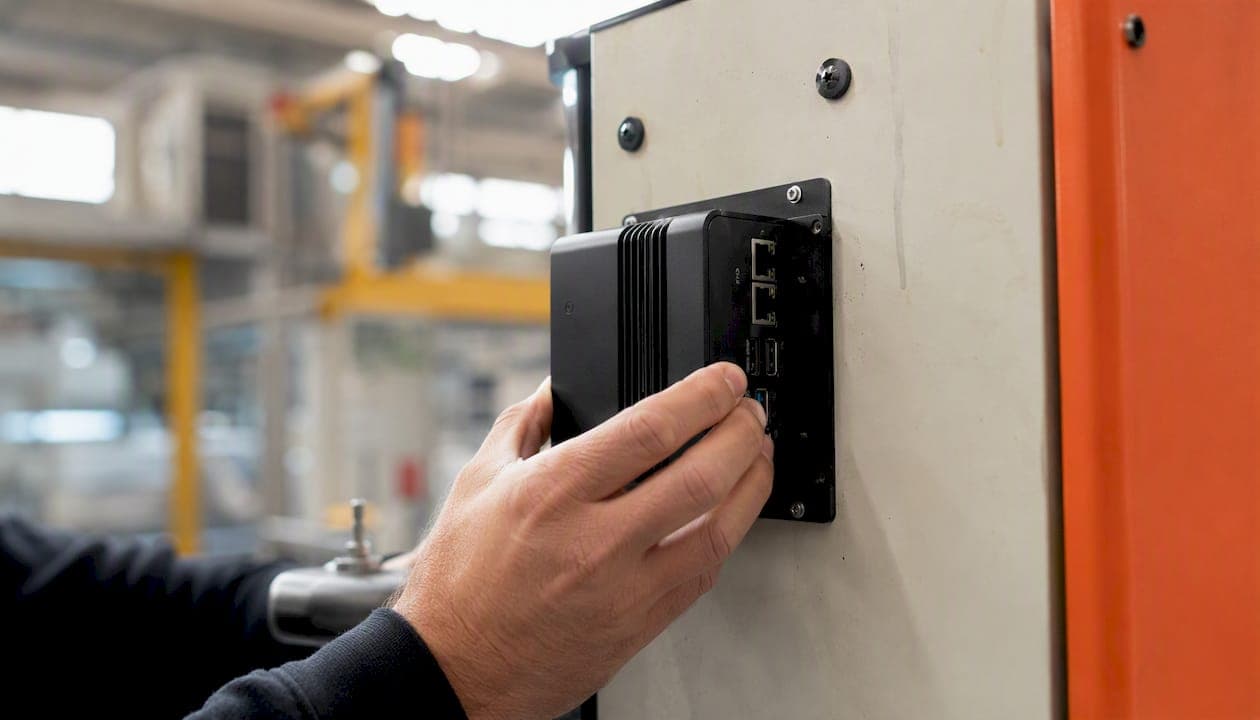
A food-processing line with limited connectivity runs a lightweight Random Forest classifier on a Raspberry Pi-class edge device. The model was trained in the cloud on labeled fault data from the same equipment type at another facility (transfer learning). Local inference runs at 1-second intervals; only anomaly flags and summary statistics are transmitted to the cloud. Full model retraining happens monthly in the cloud using accumulated edge data, and the updated model is pushed back to the edge device.
| Signal type | Common features | Example models |
|---|---|---|
| Vibration (high-rate) | Kurtosis, RMS, BPFO/BPFI FFT bins, crest factor | Autoencoder, CNN, Isolation Forest |
| Temperature (low-rate) | Rate of change, rolling mean, cross-sensor delta | Degradation model, LSTM |
| Motor current | Sideband FFT, THD, current RMS | Random Forest, XGBoost |
| Pressure | Decay rate, variance, min/max ratio | Degradation model, survival analysis |
| Acoustic emission | Energy in frequency bands, peak amplitude | One-class SVM, autoencoder |
How Arosplatforms approaches PdM pilots in manufacturing
Arosplatforms structures PdM engagements around four principles: data readiness before modeling, incremental model complexity, human-in-the-loop validation at every stage, and a clean MLOps handoff so the client’s team owns the system after deployment.
The methodology starts with a data readiness assessment on the target asset class, covering sensor coverage, sampling rates, label availability, and data quality. That assessment determines which of the three task types (anomaly detection, fault classification, or RUL) is viable in the first pilot window. Modeling begins with the simplest viable approach, typically an autoencoder or Random Forest, before introducing deep learning or hybrid architectures.
Arosplatforms clients in manufacturing have seen an average of 82% faster turnaround for key maintenance-related tasks after AI system deployment, with many programs reaching positive ROI within twelve months. The firm’s approach prioritizes ownership and scalability, meaning client teams manage their AI systems without vendor lock-in after the engagement closes.
Arosplatforms’ AI OS for Manufacturing integrates predictive maintenance with visual quality inspection and OEE analytics into a single operating layer, so PdM predictions feed directly into production scheduling and parts procurement rather than sitting in an isolated dashboard.
For organizations earlier in their AI journey, Arosplatforms’ predictive maintenance use-case page outlines typical engagement structures and outcomes across asset types.
The gap between model accuracy and operational adoption
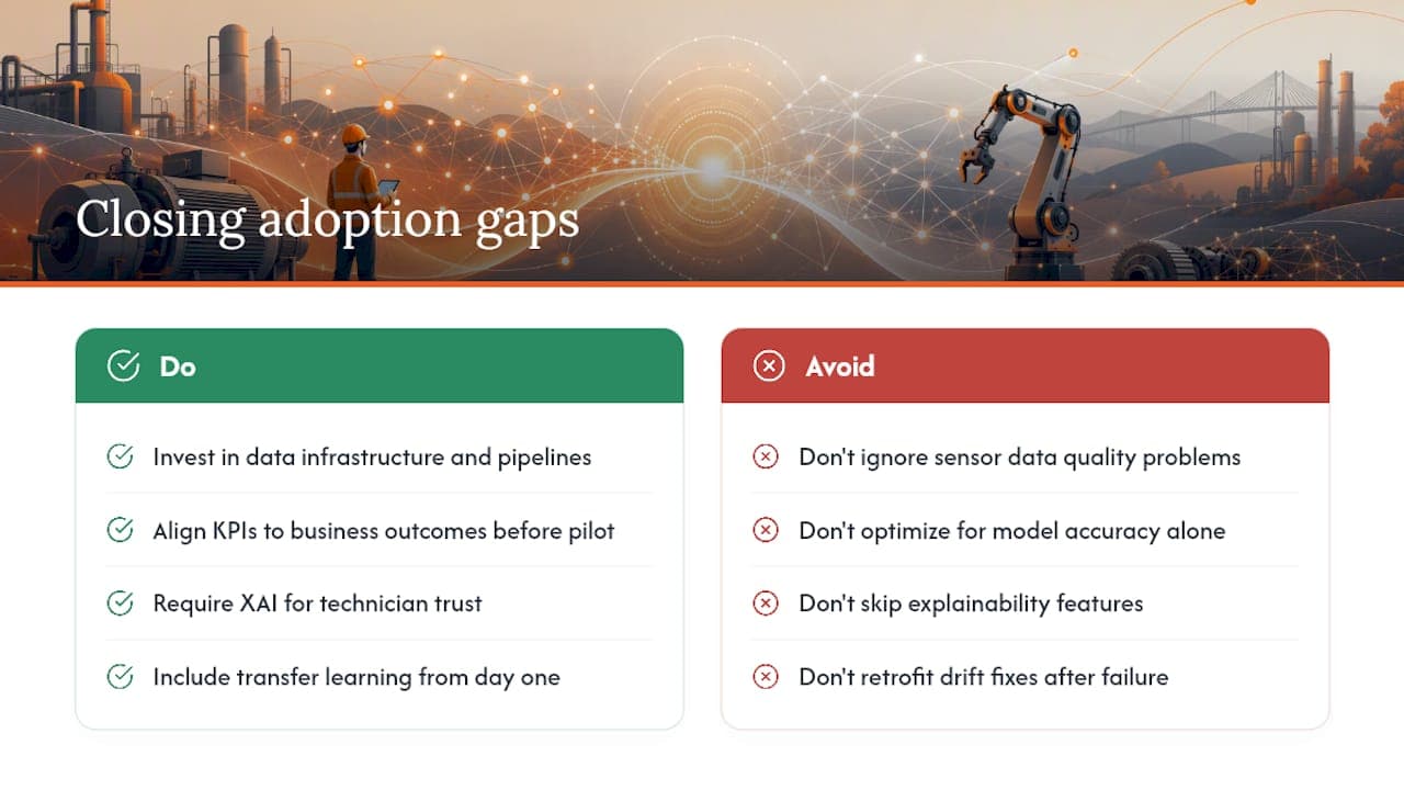
The hardest part of a PdM program is rarely the model. Most teams can train a reasonable anomaly detector within a few weeks of having clean data. What kills programs is the gap between a model that works in a notebook and a program that operations teams actually use.
Three adoption barriers show up repeatedly. First, data operations: sensor data in most plants is messier than any benchmark dataset, with gaps, drift, and undocumented maintenance events that corrupt labels. Teams that underinvest in data infrastructure spend months debugging model behavior that is actually a data problem. Second, misaligned KPIs: if the maintenance team is measured on work orders completed and the AI program is measured on model accuracy, those incentives will conflict the moment the model generates an alert the team disagrees with. Aligning on business KPIs (unplanned downtime, MTTR) before the pilot starts is not optional. Third, change management: maintenance technicians who have spent years reading machines by feel will not trust a model that cannot explain itself. XAI is not a nice feature; it is the price of adoption.
Beyond the pilot, the work that matters most is model maintenance. Concept drift in industrial settings is real and often sudden: a process change, a new supplier’s components, or a seasonal load shift can invalidate a model that was performing well. Transfer learning and domain adaptation strategies, documented in the Frontiers 2026 systematic review, are worth building into the program architecture from day one rather than retrofitting after the first drift event.
Measure success by how many unplanned failures the program prevented, not by model F1-score. The score is a development tool; prevented failures are the business outcome.
Sources
Start here depending on your immediate need:
- Predict Remaining Useful Life (RUL) - MATLAB & Simulink
- AI algorithms and IoT platforms for anomaly and failure prediction in industrial machinery—systematic review
- Survey / explainable AI for RUL (IOP)
- Building a production-ready predictive maintenance pipeline from scratch
FAQ
What is the difference between anomaly detection and RUL estimation?
Anomaly detection identifies when a machine deviates from normal behavior without specifying a failure timeline. RUL estimation predicts how much operating life remains before a defined failure threshold is crossed, expressed as a probability distribution with uncertainty bounds.
What causes AI failure prediction models to underperform in practice?
The most common causes are poor data quality (sensor gaps, undocumented maintenance events, label errors), concept drift after process changes, and insufficient failure examples for supervised training. Model choice is rarely the primary problem.
How much run-to-failure data does an RUL model need?
There is no universal minimum, but similarity models generally need at least 10–20 complete run-to-failure histories from comparable units to produce reliable estimates. Degradation models can work with fewer examples if the failure threshold is well-characterized.
Is ChatGPT or generative AI useful for equipment failure prediction?
Generative AI is not a predictive maintenance model. PdM relies on discriminative models trained on sensor data to classify faults or estimate degradation. Generative AI tools can assist with report writing, anomaly explanation drafts, or code generation for PdM pipelines, but they do not replace sensor-based prognostic models.
What is the typical ROI timeline for a PdM pilot?
Programs focused on a single high-value asset class with adequate sensor data typically reach positive ROI within 12 months, driven by reductions in unplanned downtime and emergency repair costs. Programs with more complex data requirements often take longer to achieve ROI.