Ways to Track Equipment Failure Patterns That Actually Prevent Downtime

August 17, 2026

Ways to Track Equipment Failure Patterns That Actually Prevent Downtime

Decorative title card illustration

Track failure patterns by combining canonical failure-taxonomy awareness, targeted condition monitoring, centralized time-series collection, and a layered analysis stack that moves from statistical reliability methods to root cause analysis and, where the data supports it, machine learning. No single tool does this alone. The teams that cut unplanned downtime are the ones who treat pattern tracking as a system, not a dashboard.

Run this checklist in week one:

Pull twelve months of work-order history and tag each failure by mode (bearing, seal, electrical, control).
Pick one asset class with repeat failures and assign it a single condition-monitoring technique.
Route that sensor’s output into one time-series location your team already checks daily.
Calculate baseline MTBF for that asset class before you change anything.
Set a review date 8 to 12 weeks out to compare failure rate against baseline.

Pro Tip: Start the pilot on the asset that already fails often, not your most critical asset. You want fast feedback on whether the method works, and repeat offenders give you data in weeks instead of years.

Key Takeaways

Effective failure-pattern tracking requires matching sensor type to failure mode, centralizing that data in a time-series historian, and layering statistical analysis under machine learning rather than replacing one with the other.

Point	Details
Identify the pattern first	Use the P-F curve and Weibull shape parameter to know whether you’re facing infant mortality, random, or wear-out failure.
Match sensors to fault type	Vibration, thermography, oil analysis, and motor current signature each catch different fault categories at different lead times.
Centralize before analyzing	Route all sensor and inspection data into one historian with synchronized timestamps and labeled failure events.
Prioritize with Pareto, not gut feel	Run root cause analysis only on the top 20% of repeat-failure assets, not every breakdown.
Start ML with unsupervised methods	Anomaly detection needs no labeled failure history, making it the practical entry point before supervised models.
Arosplatforms builds the connective layer	Arosplatforms designs custom AI systems that link sensors, historians, and CMMS into automated work-order triggers, with reported 82% faster turnaround on key tasks.

The Failure Patterns You’re Actually Tracking
Which Sensors Catch Which Faults
Building a Data Pipeline That Reveals Patterns
Statistical Methods That Turn Data Into Priorities
Where Machine Learning Actually Helps
Running a Pilot That Proves the Approach Works
Where Arosplatforms Fits Into Your Reliability Program
Sources
FAQ

The Failure Patterns You’re Actually Tracking

Every monitoring decision starts with knowing which failure pattern you’re dealing with, because the pattern dictates the detection window. The bathtub curve is the shorthand most reliability programs still use: high failure rates early (infant mortality), a long stretch of low, steady random failures, then a rising wear-out phase near end of life. The P-F curve matters more day to day. It plots the interval between the point a fault becomes physically detectable (P) and the point the asset actually fails (F). A bearing might give you weeks of warning through vibration; a control-board fault might give you hours. Your monitoring cadence has to match that interval, or the warning arrives too late to act on.

Reliability studies going back decades (the original work came out of aviation maintenance research) identified six recurring failure patterns, and they don’t split evenly:

Infant mortality: high failure risk right after installation or repair, then it drops.
Fatigue/wear-out: failure risk climbs steadily with age or use, classic for belts and brake pads.
Random: constant failure risk with no age relationship, common in electronics.
Slow-rise then wear-out: a gradual increase followed by a steeper climb.
Bathtub combination: infant mortality plus wear-out with a flat middle.
Pure random with no discernible pattern: the hardest to plan around, since no scheduled interval helps.

Industry reviews of aircraft and industrial equipment have repeatedly found that random-failure patterns dominate, not wear-out. That finding is the whole argument for condition monitoring over calendar-based preventive maintenance. If most of your failures don’t follow age, then replacing parts on a fixed schedule wastes money and still misses the failures that matter.

Which Sensors Catch Which Faults

Matching the sensing technology to the failure mode is where most programs either save money or waste it on the wrong equipment. Vibration analysis remains the workhorse for rotating machinery: it catches bearing wear, imbalance, misalignment, and looseness, usually weeks to months before failure. Thermography catches connection and insulation problems almost immediately, since heat shows up before mechanical symptoms do. Oil analysis reveals internal wear metal and contamination trends that no external sensor can see. Ultrasound picks up early-stage friction and electrical arcing that vibration sensors miss entirely. Motor current signature analysis reads the electrical waveform to catch rotor bar and stator issues without opening the motor.

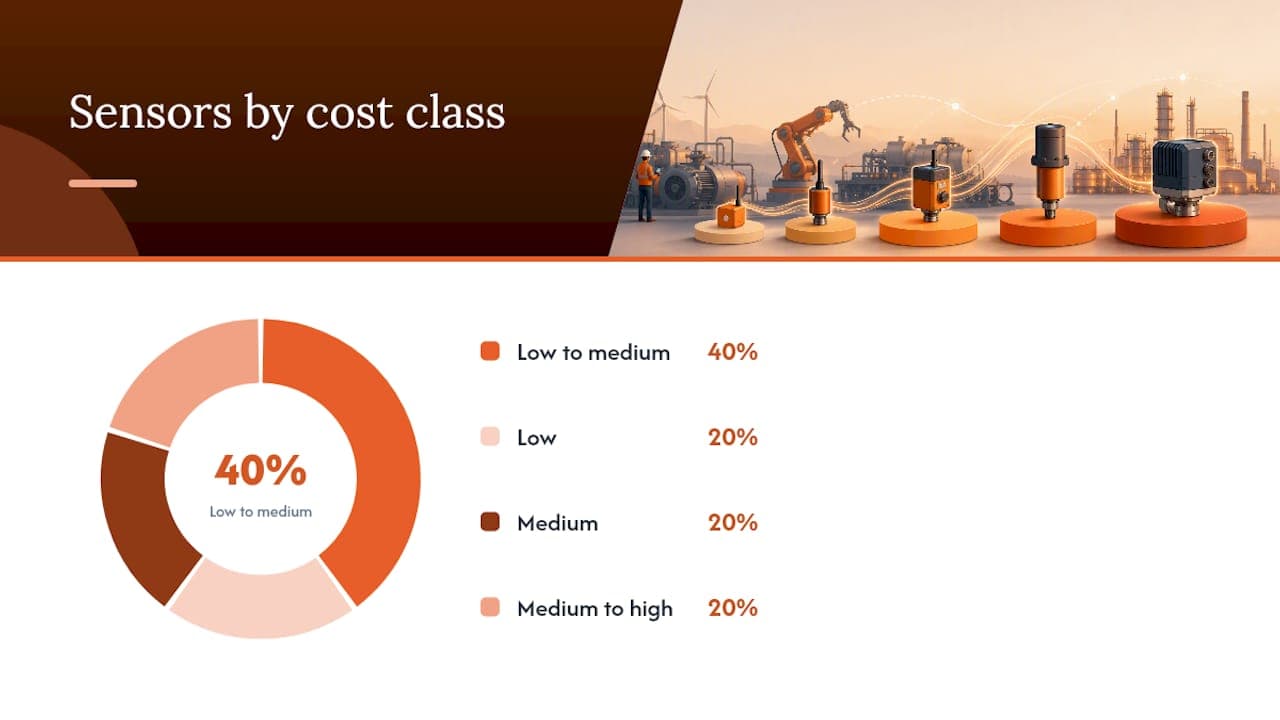
Technique	Detects	Typical Cadence	Cost Class
Vibration analysis	Bearing wear, imbalance, misalignment	Continuous or monthly route	Low to medium
Thermography	Loose connections, insulation breakdown	Quarterly or continuous	Medium
Oil analysis	Internal wear metals, contamination	Monthly to quarterly	Low
Ultrasound	Early friction, electrical arcing, leaks	Monthly route	Low to medium
Motor current signature	Rotor/stator faults, electrical imbalance	Continuous or annual	Medium to high

Comparison diagram of sensor types and detected faults

Portable inspection routes make sense for lower-criticality assets where a monthly check is enough warning. Permanent sensors earn their cost on assets where the P-F interval is short or the failure consequence is severe enough that a missed monthly reading is a real risk.

Pro Tip: Don’t rely on one signal for critical assets. Combining vibration with thermography or oil data (data fusion) cuts false positives dramatically, because a single sensor drifting out of range looks very different from two independent signals trending the same direction.

Building a Data Pipeline That Reveals Patterns

Sensors are useless if the data dies in a spreadsheet nobody opens. The practical architecture looks like this: edge devices capture raw signal, local logic filters noise and flags obvious outliers, a time-series historian stores the cleaned data, an analytics layer runs trend and threshold logic, and the results feed your CMMS as work orders or alerts. Historian storage paired with FFT and envelope analysis is what turns raw vibration waveforms into usable trend alarms instead of noise.

Before any of that produces trustworthy patterns, check these:

Timestamps are synchronized across every sensor and system, not just internally consistent.
Sampling rates match the fault frequency you’re trying to catch, not a generic default.
Every reading carries operating-context metadata: load, speed, ambient temperature.
Failure events are labeled at the moment they happen, not reconstructed weeks later from memory.

Pro Tip: Label failures the day they occur, including near-misses. Reconstructed failure timelines from memory are consistently wrong on the exact date, and that error alone can wreck a Weibull analysis.

Statistical Methods That Turn Data Into Priorities

Weibull analysis is the backbone of quantitative failure pattern work, and it’s worth learning even if you never run the math by hand. The shape parameter tells you which failure pattern you’re in: a shape value below 1 signals infant mortality, near 1 signals random failure, above 1 signals wear-out. The scale parameter estimates characteristic life. Run it on censored data (assets still running, not yet failed) when you can, since ignoring survivors biases your estimate toward pessimism.

MTBF and MTTR do simpler, faster work. MTBF (mean time between failures) tells you how often an asset class fails; MTTR (mean time to repair) tells you how long each failure costs you. A pump averaging 2,000 operating hours between failures with a 4-hour repair time has a very different maintenance profile than one failing every 500 hours with an 8-hour repair, even if both look “problematic” on a work-order count alone.

Once you have both numbers, prioritize root cause work this way:

Run a Pareto count of failures by asset and mode over the past 12 months.
Isolate the top 20% of assets driving roughly 80% of failure events.
Run structured FMEA only on that top tier, not every breakdown.
Assign corrective action with an owner and a deadline.
Re-measure MTBF after 90 days to confirm the fix held.

Where Machine Learning Actually Helps

Machine learning earns its place once you have enough labeled failure history to train on, and not much sooner. Supervised models need labeled fault examples and work well when you have years of tagged failure data. Unsupervised anomaly detection needs no labels at all. It flags deviations from normal operating behavior, which makes it the practical starting point for most plants, since labeled failure data is almost always scarce. Hybrid approaches, blending physics-based models with data-driven learning, tend to generalize better with less labeled data while staying interpretable enough for safety-critical assets.

The results can be striking. Frequency-domain vibration image techniques have reported 99.4% classification accuracy for incipient faults, and unsupervised novelty detection in that same research located developing faults up to three days before total failure. That’s real, but read it carefully: three days of warning is useful for a rotating asset with a slow-developing bearing fault, and nearly useless for a fast electrical failure. Model-based detection stays more interpretable than pure data-driven approaches, which matters when a maintenance planner needs to explain a recommendation to a plant manager.

Before deploying any model, check:

A genuine train/test split with data the model has never seen, not a lucky subset.
Ongoing monitoring for concept drift as operating conditions change seasonally.
An explainability threshold appropriate to asset criticality (a conveyor belt tolerates a black-box model; a pressure vessel doesn’t).

Comprehensive reviews of data-driven fault diagnosis consistently find that models trained on one plant’s conditions generalize poorly to another’s, so validate on your own asset data before trusting the number.*

Running a Pilot That Proves the Approach Works

A good pilot answers one question in under three months: does pattern tracking on this asset class reduce failures or catch them earlier? Keep the scope tight.

Pick one asset class with a documented repeat-failure history.
Deploy one or two sensing techniques matched to the known failure mode.
Set a baseline MTBF using the past 12 months of work orders.
Define success in advance: a specific percentage reduction in unplanned failures, or a target number of early-warning catches.
Integrate alerts directly into your CMMS so the pilot doesn’t depend on someone remembering to check a dashboard.

Assign roles clearly: a maintenance lead who owns the asset relationship, a data or reliability engineer who owns the historian and models, and if you’re bringing in outside expertise, a consultant who owns integration with existing predictive maintenance workflows.

Weeks 1 to 2: install sensors and confirm data flow.
Weeks 3 to 8: collect baseline data, no changes to maintenance behavior yet.
Weeks 9 to 12: act on the first flagged anomalies and log outcomes.

Vendor case reporting on AI-driven condition monitoring has cited avoided downtime in the hundreds of hours and six-figure savings on prevented equipment replacement in specific customer examples. Treat those as directional evidence of what’s possible, not a guaranteed outcome for your plant.

What I’d Tell a Team Starting This Tomorrow

Don’t run root cause analysis on every breakdown. Run the Pareto first, then dig deep only on repeat offenders; everything else gets a quick fix and a log entry. Use model-based detection for well-understood mechanical failures where physics gives you a head start, and save data-driven ML for the messy, high-volume asset classes where nobody has written the physics down yet.

Hands wiring industrial control panel

Where Arosplatforms Fits Into Your Reliability Program

Most maintenance teams don’t lack sensors. They lack a system that connects those sensors, the historian, the CMMS, and the analysis layer into something that actually triggers a work order before a failure happens. Arosplatforms builds that connective layer as a custom AI operating system, embedded directly into your existing maintenance stack rather than sold as another dashboard to check. That means the anomaly a vibration sensor flags at 2 a.m. can route straight into a work order, with no manual handoff and no dashboard nobody opens.

Hands connecting sensor cables to machinery

Clients working with Arosplatforms typically see 82% faster turnaround on key maintenance tasks, with ROI often visible inside the first twelve months. If you’re a US-based manufacturing or industrial operation ready to move from scattered sensor data to a working predictive maintenance pipeline, Arosplatforms’ US consulting team can scope a pilot around the asset class you already know is causing the most repeat failures. Start with a conversation about that one asset, not a plant-wide overhaul.

Sources

FAQ

What are the different types of failure modes in equipment?

Common failure modes include bearing wear, misalignment, imbalance, seal degradation, electrical insulation breakdown, and corrosion, and each tends to follow one of the six canonical failure patterns like infant mortality or wear-out. FMEA frameworks are the standard way to catalog these modes by asset type and rank them by severity and detectability.

How do you keep track of equipment maintenance?

Centralize work orders, inspection results, and sensor data in a CMMS linked to a time-series historian, so failure history, MTBF trends, and condition-monitoring alerts live in one searchable system instead of scattered spreadsheets. Consistent labeling of failure events at the time they happen is what makes that history usable for later analysis.

How do you perform a failure analysis?

Start with a Pareto count of failures by asset and mode to find repeat offenders, then run a structured root cause analysis (often paired with FMEA) only on the highest-impact assets, followed by a corrective action with a defined owner and a recheck of MTBF after the fix. Statistical tools like Weibull analysis add rigor by identifying whether the failure trend is random, wear-out, or early-life.

What are some examples of failure modes?

Bearing spalling, motor winding insulation failure, seal leakage, coupling misalignment, and lubrication breakdown are frequent examples across rotating equipment, each detectable through a specific monitoring technique such as vibration analysis or oil analysis. A predictive maintenance program built around these known modes, like the frameworks Arosplatforms designs for manufacturing clients, ties detection directly to a work-order trigger instead of a static alert.

Ways to Track Equipment Failure Patterns That Actually Prevent Downtime